 |
It is very easy to correct a digitized signal for droop:
 |
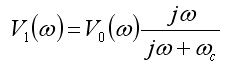
Often, a measured signal, V1, will have a droop
associated with an RC or L/R decay time. This is equivalent to the
desired signal, V0, being sent through a
high-pass RC filter before being recorded:
|
 where,

|
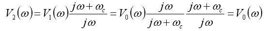
To get the desired signal back, we need to multiply by the inverse
of the high-pass RC filter transfer function and generate a droop
corrected signal, V2: |
|
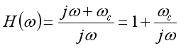
So, the correction in the frequency domain, H(ω),
is: |
|
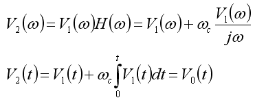
Because of the linearity of the Fourier transform and recognizing
that division by jω in the frequency domain is
integration in the time domain: |
|
So, it turns out that this correction is nearly trivial to make with
a computer code:
 |
For (i=0; i<NumberOfPoints; i++)
{
Integral+=v1[i]*TimeStep;
v2[i]=v1[i]+Integral/RC;
};
|
|
|
